Classifying Supernovae

This is a project for the ASTR 230: Astronomy Laboratory at Rice University. I attempt to classify supernovae using instrumental magnitudes from the Hα, V, and R filters at the 0.8 meter telescope at McDonald Observatory.

There are two different types of supernovae, type 1 and type 2. The main distinguishing factor between the two of them is that type 2 has hydrogen lines and type 1 do not. This is because the type 2 supernovae still have a hydrogen envelope around them, while the type 1 have lost theirs in some way. However, there are some similarities in how the two types of supernovae occur.

The type 1B, type 1C and type 2 supernovae are formed when a supergiants's core collapses and the resulting shock wave causes them to explode into a supernova. The type 1A supernovae are also known as standard candles. They're white dwarves in binary systems where they are continuously stealing matter from their companion. Eventually, they gain so much mass that they exceed the Chandrasekhar limit, at which point they are no longer able to sustain themselves using electron degeneracy. Fusion starts in their core and the dwarf explodes in a type 1A supernova.

Even though the type 1 supernovae have different evolution paths, they all have one thing in common: a lack of hydrogen lines. The result that I expect when I compare the Hα/R ratios of the type 1 and type 2 supernovae is that the type 2 supernovae will have a significantly higher ratio than the type 1 supernovae. I also included the V/R ratio, in case it may be another factor. However, I do not expect there to be a significant difference.

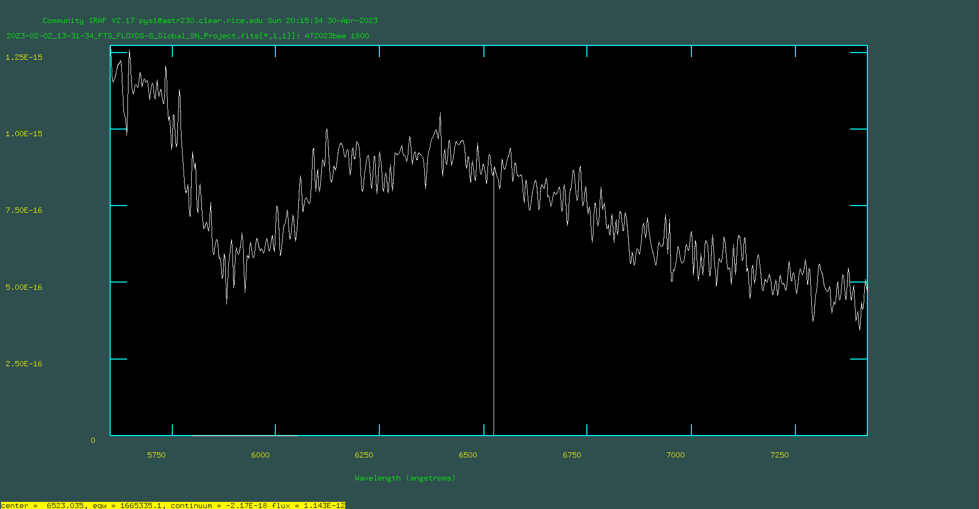
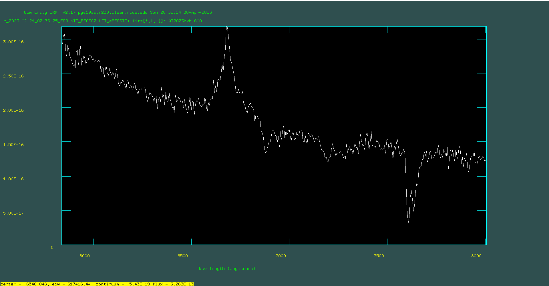
In order to test this, I took the spectra of a typical type 1 and type 2 supernova and integrated the flux in IRAF within the R and Hα bandpasses I used. I chose supernovae with z < 0.02 so that the redshift would minimally affect the integration. As you can see below, the type 2 supernova has a strong Hα line where the type 1 does not. I centered my integration at the location of the Hα line at 6563 Å. The R bandpass estimate that I used was 1600 Å wide, although the actual bandpass was closer to 1200 Å wide. The Hα filter at McDonald that I used was 700 Å wide, but I also integrated the flux for a 200 Å wide bandpass as that is the width of the filter that we have on hand at Rice University. I did the integration for both to see if the narrower bandpass would help isolate the Hα line more.

After doing my flux integration in IRAF, the Hα/R ratio that I got for the wider R bandpass for the type 1 supernova was 0.505 and for the type 2 was 0.457. However, with the narrower bandpass I got 0.142 for the type 1 and 0.150 for the type 2. It is likely that because the McDonald R bandpass is so wide, the Hα line is being averaged out so that it doesn't change much in the ratio. The Hα line may look very wide in the spectra above, but that is because it is very zoomed in. With such a large bandpass it's not going to make as much of a difference in counts as I'd want it to. But with the narrower filter, I was able to get results that lined up more with what I expected, which is that the type 1 has a lower Hα/R ratio than the type 2. These supernovae were also part of my dataset, so as shown in the next section these Hα/R ratios are reflected in the actual data I analyzed.

I got data for 8 different supernovae: four type 1, three type 2, and one of unknown type. Only using the McDonald telescope was very helpful for me, because normally I would need to compare the actual magnitudes of the different supernovae. However, since I was just using the same telescope and comparing only within the same object, I only need the ratios within the object. I was able to just use the counts and avoid using any standard stars to calculate the magnitude, which allowed me to skip a lot of extra steps when reducing my data. The only extra thing I had to do with make sure that I normalize my counts for the exposure time. Most of the images that I took had an exposure time of 180 seconds, but then some of the earlier ones I was a little too cautious about oversaturating 15th magnitude objects so I kept my exposures short at only 15 or 60 seconds. Since counts increase linearly with time, normalizing the counts is a quick arithmetic operation.

The most crucial part of this whole project was determining what the background sky value was for each supernova. I had to look at each and figure out what do I believe could be the background value. I used three different values for my background: the one I thought was the most likely candidate for the background, the minimum possible one that I could believe, and the maximum possible that I could believe. I used the minimum and maximum values for the error bars in my plot, and the middle value as the data point.

Some of them are really easy. They were just kind of floating out in the star field, nothing around them. It was very easy to figure out the sky values for those. However, some of them were in galaxies which made things a lot more complicated because galaxies have complicated structure. There's arms and gaps and clumps in the arms that are brighter and darker, so I had to be really careful about the location of each supernova.

All of this had to also be done by hand. I cannot have the computer do this for me because of all the complexities, especially in the galaxy. I manually went into DS9, made a little region, and explored around the supernova and then decided by looking at the mean and medians what I think is noise and what I think is actually meaningful.

For the last bit for data reduction after I subtracted out my sky values, I used IRAF for photometry. I manually input the apertures and coordinates. I didn't want IRAF to start trying to calculate things for me, because it tries to calculate the location of the star itself and then ends up doing photometry on the core of the galaxy, which gives very different results than the tiny little supernova on the arm. To avoid this, I had to turn off all any auto fitting that IRAF tries to do.

Once I had my apertures set and looked at the data that came out I chose the aperture for each supernova that I think is most correct. This was based on when the counts start to either plateau or maxed out. Once the counts start to plateau, that's when the aperture has passed the edge of the supernova and nothing else is contributing to your photometry except the sky, which has been zero-d out.

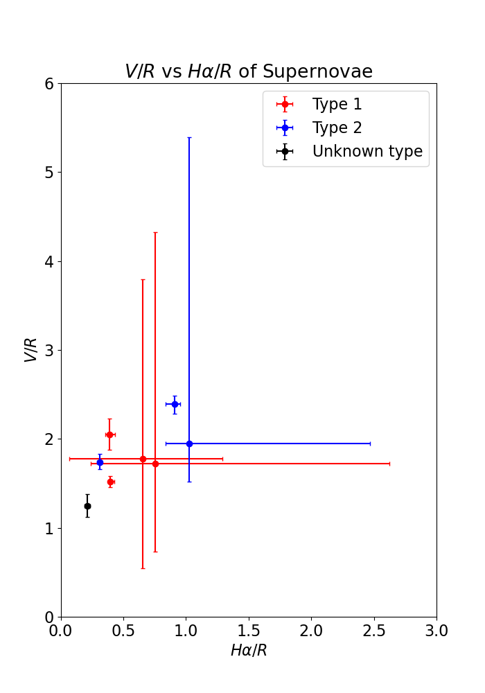
For my statistical analysis, I performed a two sample t-test because I have two independent populations with a very small sample size. The p-value that I got from the two populations' Hα/R ratio was 0.3936 and for the V/R ratio was 0.2654. This is not statistically significant and I cannot reject my null hypothesis that the two populations have different average ratios. However, just looking at the plot we can say that the unknown type supernova is most likely a type 1 supernova and that 2023bvh may be an outlier.

2023bvh was actually one of the spectra I used that I thought was a typical type 2 supernova. It had an unmistakable Hα line but as we can see here, the ratio is quite low. This supernova was on the edge of a galaxy but I was still confident in the sky values as seen by the low err bars, so I can't attribute the low counts to it being in a galaxy. However, the flux ratio is comparable to as we predicted it would be in the Expected Results section. Additionally, if we do treat it as an outlier, the t-test that I discussed earlier leads to a p-value less than 0.05, which means that there is a statistically significant difference between these two populations. This means that I can be more confident in my conclusion that the unknown type supernova 2023dpm is a type 1. But this is only if it's an outlier, which I'm not convinced about just because it had such a strong Hα line.

The way I calculated the error bars is such that it's the maximum and minimum possible ratios you can get with the sky values I subtracted. The very large error bars on three of my data points are due to the fact that it is very difficult to estimate the sky value inside a galaxy. However, The values that I got for Hα/R from what believe is the correct sky value are below 1.0, which is as expected. Hα can't be bigger than R because the Hα bandpass a subsection of the R bandpass.

I originally expected the type 2 supernovae to have much higher Hα/R ratios than the type 1 supernovae. I also wasn't really expecting much of a correlation to be in V/R, which was what my results did show. However, I was unable to determine statistical significance for the Hα/R ratios without throwing out one of my data points as an outlier. Even though the difference between the two samples was not statistically significant, I believe that the unknown type has such low Hα/R that I can still make an educated guess that it is a type 1 supernova.

One of the main weaknesses in this project is that I did not get nearly enough data to perform a proper statistical analysis. This is due to the fact that each data point requires at least one image per filter, often going up to three images each depending on magnitude. Many of my objects were very faint, so this took up a lot of telescope time.

Spectra appears to be much more effective at classifying supernovae than images, just due to the fact that something that is so obvious in spectra might not show up in imaging. The narrower Hα filter would do a better job of isolating the Hα line and reducing interference from other objects. In a wide bandpass, the Hα averages out to be just a little blip that doesn't affect the Hα/R ratio.

Carini, R., Ragosta, F., Benetti, S., Reguitti, A., & Yaron, O. (2023). ePESSTO+ Transient Classification Report for 2023-02-21. Transient Name Server Classification Report, 2023-407, 1.

Carroll, B. W., & Ostlie, D. A. (2017). An Introduction to Modern Astrophysics. Cambridge University Press.

Gal-Yam, A., Mazzali, P. A., Manulis, I., & Bishop, D. (2013). Supernova Discoveries 2010-2011: Statistics and Trends. Publications of the Astronomical Society of the Pacific, 125(929), 749-752. doi:10.1086/671483

Harvey Mudd College Astronomy. (n.d.). CCD reduction. Photometry in IRAF. Retrieved April 23, 2023, from http://www.physics.hmc.edu/Astronomy/Ireduce.html

Zhai, Q., Zhang, J., Li, L., & Wang, X. (2023). LiONS Transient Classification Report for 2023-02-01. Transient Name Server Classification Report, 2023-260, 1.